DHR/AR Rheometer: Calibrating a Geometry
Overview
There are geometry-specific calibrations that are performed from the Calibrations tab on the document view of the current geometry. To access this view, use any of the following techniques:
- Select Home tab > Geometry toolbar > Edit.
- Select Instrument tab > Calibrate > Geometry calibrations.
- View the geometry with a green check mark on the Geometries section of the File Manager and select Calibrate.
A yellow warning triangle  or green check mark
  indicates the current status of each of the available calibrations. Once a calibration has been performed, the value is recorded together with the time and date. The validity of some calibrations are time-based and will revert to the warning triangle state after this time period has elapsed.
Back to top
Geometry Inertia Calibration
Ideally, whenever a stress is applied by a rheometer, it acts solely upon the loaded sample and nothing else. In practice, however, the non-zero moments of inertia of the rheometer spindle and measurement geometry mean that some of the applied torque is being used to accelerate or decelerate these mechanical components (until steady state is reached.) A correction needs to be made to the stress value to reflect more accurately the conditions that the sample is undergoing. The amount of correction applied is based upon the calibrated values of the instrument and geometry inertia.
This calibration only needs to be performed once per geometry. The total moment of inertia (instrument + geometry) is an important parameter in the calculation of oscillatory data, and correcting controlled stress flow ramps (oversampling off). It is also an important parameter for optimal controlled rate control and creep recovery breaking.
In the oscillation mode, the correction is made automatically. In the flow mode, however, the correction can be toggled on or off as necessary. Flow inertia correction is more likely to be needed when low-viscosity materials are being measured using fast ramps over a wide shear range.
To calibrate the geometry inertia, expand the Inertia calibration area, follow the instructions, and click Calibrate. When complete, you can Accept or Cancel the new value.
Back to top
Friction Calibration
AR bearings provide virtually friction-free application of torque to the sample. However, there will always be some residual friction. With most materials, this is insignificant; but for low-viscosity samples, this inherent friction causes inaccuracies in the final rheological data. To overcome this, the software has a friction correction that can be activated, if required. This value changes slightly with geometry and is a torque correction, based on the angular velocity, that is made to flow data.
To calibrate the friction, expand the Friction calibration area, follow the instructions, and click Calibrate. When complete, you can Accept or Cancel the new value.
Back to top
Compliance Calibration
Unless the stiffness of the sample approaches the stiffness of the geometry and rheometer drive shaft, a correction for compliance can generally be ignored. A compliance value appropriate for the geometry/rheometer/temperature system combination is automatically entered by the software, but in the case of torsion geometries, it is possible to perform a unique calibration.
To calibrate the compliance for torsion geometries, expand the Compliance calibration area, clamp the short compliance sample supplied in the torsion kit between a matched set of clamps, and click Calibrate. When complete, you can Accept or Cancel the new value.
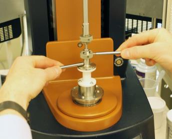
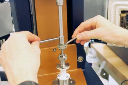
To load the torsion cylindrical compliance sample:
- Fit the 4.5 mm collets, attach the upper geometry and zero the gap.
- With the upper geometry removed insert a Tommy Bar into the lower hole in the lower assembly and drop in the steel rod.
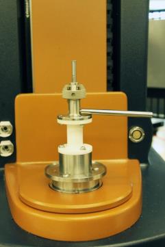
- Fit the upper geometry, and then lower the head so that the rod can be guided into the collet.
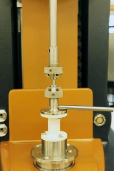
- Finger tighten both clamps, before using the Tommy Bars as shown in the pictures below.
- Warning: Using a single Tommy Bar to tighten either collet could result in fracturing the ceramic heat break.
Back to top
Gap Temperature Compensation
In general isothermal operation, a geometry is zeroed at the test temperature and then the measurement gap set from this reference point. However, if the temperature is then changed, there will be a commensurate change in the measurement gap due to the thermal expansion/contraction of the upper and lower geometries. This results in erroneous calculations of rheological properties unless an appropriate correction is made. This correction is most useful for procedures where measurements are made at different temperatures without reloading the sample (for example, temperature ramps and temperature sweeps).
The correction can be toggled on or off as necessary. When active, there are two modes of operation, depending on the axial force control.
- When axial force control is not active, the rheometer head physically moves to maintain the initial measurement gap using the gap temperature compensation value. The gap reported in the results file will be within a few microns of the initial gap.
- When axial force control is active, the rheometer head physically moves to maintain the initial measurement gap as long as the movement of the head does not result in an axial force that exceeds the control value specified. Once this occurs, the reported gap is modified by the gap temperature compensation value, so the gap reported in the results file will be the corrected gap.
To calibrate the gap temperature compensation, expand the Gap Temperature Compensation calibration area, follow the instructions, complete the settings that are appropriate for your test, and click Calibrate. When complete, you can Accept or Cancel the new value.
Back to top
Rotational Mapping (DHR Series)
Any bearing will have small variations in behavior around one revolution of the shaft. They are consistent over time unless changes occur in the bearing. By combining the absolute angular position data from the optical encoder with microprocessor control of the motor, these small variations can be mapped automatically and stored in memory.
These variations can then be allowed for automatically by the microprocessor, which is in effect carrying out a baseline correction of the torque. This results in a very wide operating range of the bearing.
There are three levels of rotational mapping – fast, standard, and precision. It is also possible to perform multiple mappings (iterations).
When should you use rotational mapping? The magnitude of the torque correction varies with the instrument type, but typically has an absolute maximum in the range 0.2 to 1 µN.m. With this in mind, you can determine if mapping will improve your measurements. For example, if the minimum torque during your procedure never drops below 100 µN.m, then the maximum error that an unmapped bearing will contribute is 1%. In this case, you may consider that mapping is not required or that a fast mapping is sufficient. As the torques in your procedure drop, the error from an unmapped bearing increases, so it may become necessary to perform precision mappings to keep these errors to a minimum.
For optimum performance at very low torques, multiple mappings can be performed, but there are diminishing returns. Generally, you will see little further improvement in performance after three consecutive mappings.
For maximum accuracy at the lower torque end of the rheometer, it is recommended that the mapping be performed each time a new measuring system is used, or if the current geometry is removed for cleaning.
To calibrate the Rotational Mapping:
- Access the Rotational Mapping panel.
- Expand the Calibration area of the Rotational Mapping panel.
- Select the type of mapping and number of iterations.
- Click Calibrate.
- NOTE: The mapping is remembered by TRIOS software if the instrument is powered off. The mapping is also remembered following a service bearing test.
Back to top
Axial Mapping (DHR Series)
The performance of small amplitude axial oscillation tests is directly related to the control of the magnetic bearing, which supports the upper geometry. The axial mapping linearizes the displacement output of the magnetic bearing and measures the mass of the upper geometry, needed to correct for instrument inertia contributions.
Since the mass of each upper test fixtures varies, axial mapping has to be performed for each upper test fixture that is used for axial oscillation testing. The available displacement range is from +/- 1 to 100 micron. The axial mapping is saved in the geometry file and is reloaded when the geometry is reinstalled. For maximum accuracy it is however recommended that the mapping be performed each time a new measuring system is installed.
To calibrate the Axial Mapping:
- Install the desired test geometry (see also Available Test Geometries)
- Make a geometry active by loading the geometry file from the experiment ribbon or generate a new geometry file (see also Configuring a New Geometry).
- Click on the active geometry in the geometry list in Geometries of the File Manger Navigation panel to open the Calibration tab.
- In the Axial Mapping section, select the following:
- Read Alignment Position: The instrument reads the current home position for the upper geometry.
- Calibration (using existing alignment position): Use this tab to map a geometry that has been installed. Note that calibration is only possible after an alignment position has been definied.
- Click Calibrate.
- NOTE: The axial mapping is remembered by TRIOS software if the instrument is powered off. The mapping is also remembered following a service bearing test.