| Introduction |
| List of Available Transformations |
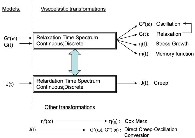
In TRIOS, rheological transformations are operations executed on experimental and calculated data to convert one data file into another (for example, the conversion of the Relaxation Time Spectrum data file into a Relaxation or Oscillation data file). Transformations in TRIOS always operate on complete data files when launched from the File Manager menu.
Transformations are divided into two groups: 1. Viscoelastic transformations and 2. Other transformations. All transformations available from TRIOS are shown below.

Viscoelasticity transformations:
Relaxation time spectrum --->Oscillation (G*, G’, G”, δ*)
Relaxation time spectrum ---> Relaxation (G(t))
Relaxation time spectrum --->Stress Growth (η(t))
Relaxation time spectrum --->Memory function (m(t-t’))
Relaxation time spectrum ↔Retardation time spectrum
Retardation time spectrum --->Creep (J(t))
Other transformations:
Cox-Merz (η*---> η(g))
Fluid Inertia Correction
Rabinovicz Correction
Direct Creep – Oscillation conversion (J(t)---> G’, G”)
Discrete Fourier Transformation (DFT) for general temporal strain and stress data sets
Window Correlation
Temperature Ramp ---> Frequency ramp at explicit temperature
Frequency Ramp ---> Temperature ramp at explicit frequency
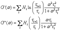
This transformation converts the discrete/continuous relaxation spectrum to oscillation data G’, G”, G* and η*.
The discrete relaxation spectrum {Gi;ti}is used to reconstruct the parameters G’ and G” for the user selected frequency range according to:

G’ and G” are reconstructed from the continuous relaxation spectrum{Hi; ti} according to:
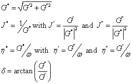
Other dependent variables are calculated as:
Note that an average temperature is recovered from the original experiment file and saved with the reconstructed data.
This transformation converts the discrete/continuous relaxation spectrum to the relaxation modulus G(t).
The discrete relaxation spectrum {Gi;ti} is used to reconstruct the relaxation modulus in the user selected time range according to:

G(t) is reconstructed from the continuous relaxation spectrum{Hi; ti} according to:

The stress is also computed based on a user selectable strain (default 100%).
Note that an average temperature is recovered from the original experiment file and saved with the reconstructed data.
This transformation converts the discrete/continuous relaxation spectrum to the viscosity function η(t) and the normal stress coefficient ΨΛ(t).
The discrete relaxation spectrum {Gi;ti} is used to reconstruct the viscosity function in the user selected time range according to:

h(t) and y1(t) are reconstructed from the continuous relaxation spectrum{Hi; ti} according to:
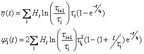
The shear and the normal stress are also computed based on a user selectable strain rate (default 1).
Note that an average temperature is recovered from the original experiment file and saved with the reconstructed data.
This transformation converts the discrete/continuous relaxation spectrum to the memory function m(t-t’).
The discrete relaxation spectrum {Gi;ti} or the continuous relaxation spectrum{Hi; ti} is used to reconstruct the viscosity function in the user selected time range according to:

Note that an average temperature is recovered from the original experiment file and saved with the reconstructed data.
This transformation converts the discrete/continuous retardation spectrum to the compliance J(t).
The discrete retardation spectrum {Ji;ti} or the continuous relaxation spectrum{Li; ti} is used to reconstruct the compliance in the user selected time range according to:

The strain is computed also, based on a user selectable stress (default 1).
Note that an average temperature is recovered from the original experiment file and saved with the reconstructed data.
The transformation of Relaxation to Retardation time spectrum and vice versa is key for converting relaxation to creep data. Conversion between the complementary (i.e. retardation and relaxation) discrete or between the complementary continuous spectra can be made. Numerical methods have to be used for the conversion between continuous spectra, whereas the discrete spectral conversion is exact. The conversion of the continuous spectra is as follows:
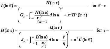
The conversion of the discrete retardation to relaxation spectrum involves the following steps: The discrete relaxation times ti are the roots of the equation:

The magnitude Gi is calculated as:

For the conversion of the discrete relaxation to retardation spectrum, the discrete retardation times ti are the roots of the equation:

The magnitude Ji is calculated as:

The Cox-Merz "rule" is an empirical relationship that has been found to be of great use in rheology. It was observed by Cox and Merz that for many polymeric systems, correspondence occurred between the steady state shear viscosity (plotted against shear rate) and the magnitude of the complex viscosity (plotted against angular frequency). The complex viscosity is defined by:

If applied correctly, the Cox-Merz rule can be of great value in polymer rheology, and there are several circumstances in which it might be used.
The Cox-Merz rule has been found to hold for almost all polymer melts, and concentrated and semi-dilute solutions. Deviations from the rule occur at high frequencies, and the oscillatory data can either over- or under estimate the steady state data. Instances of polymeric systems for which it has been found not to apply are Boger fluids and certain other dilute solutions, and cross-linked or gelled systems. The rule also fails for most particulate dispersions.
The usefulness of the Cox-Merz rule has led to similar expressions between the first normal stress difference, N1, and G’:
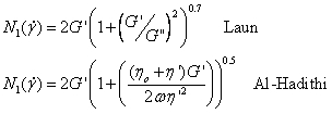
These expressions should be applicable to at least those systems for which the Cox-Merz rule holds. It is an acknowledged weakness that a value for ηo has to be inserted in the Al-Hadihti equation or at least determined parametrically. In TRIOS, ηo is obtained by fitting a Williamson model to the oscillatory data.
Most rheological measurements are made under the assumption that the fluid inertia is negligible. Neglecting fluid inertia can result in measurement errors of both the viscosity and phase angle. Fluid inertia is negligible when the wavelength λ of the propogating sine wave is much longer than the sample gap. The fluid in the gap only sees a small portion of the wave propagation.
If the shear wavelength λ is of the same order of magnitude than the gap, the amplitude and the phase of the velocity gradient are a function of the position within the gap. The phase of the strain rate at any point lags the strain rate at the driven surface.
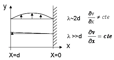
For small amplitude oscillation the velocity in the shear plane is given by the equation of motion

with the following boundary conditions:
x=0 (stationary surface): v(0,t)=0
x=d (moving surface) v(d,t)=v0exp(iωt)
At any distance x within the gap, the velocity is:

The velocity gradient at the stationary surface x=0 (geometry attached to the transducer on the ARES, geometry attached to the base on AR) with Γ=(iρω/ η*)0.5, is:

The stress at the stationary surface is:

Defining the apparent shear rate  a(t) (assuming constant shear rate in the gap)

and dividing the stress equation with the  a(t) gives:

Since G*a=iω η*a and G*=iω η*

This equation has to be solved for G* using the measured apparent modulus G*a as starting value.
The corrected storage and loss modulus are obtained from G*=G’+iG” and the correct phase from δ=arg(G*)
Since this equation is solved by an iterative process, it is unpractical to perform the fluids inertia correction in real time and has therefore been implemented as a transformation. [G. Böhme and M. Stenger, J. Rheal. 34, 415 (1990)]
To limit the magnitude of the correction, it is good practice to minimize, where practical, the size of the gap used in the measurement of very low viscosity fluids.
The phase reported is calculated as:
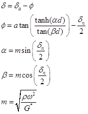
The complex viscosity is computed as:
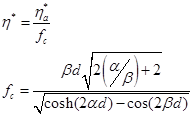
The real time fluids inertia correction and the post correction are active when the material parameter density is a non zero value. When the fluids inertia correction transformation is applied to a data set, the previously performed real time correction is reset.
Fluids inertia correction is only performed when parallel plate and concentric cylinder geometries are used.
In parallel plate geometry, in wide gap Concentric Cylinder and Poiseuille flow geometries, the shear rate is not a constant. The shear rate in parallel plate geometry for example is zero in the centre and maximum at the rim.
If the geometry for parallel plate is selected, the stress is calculated from the measured torque at the maximum shear rate at the rim radius R. For non-Newtonian fluids, the stress is a function of the shear rates(g) and the computed stress is an apparent stress. In order to obtain the true stress, the stress needs to be corrected for the strain rate dependence.
The torque balance in parallel plate geometry can be written as:

Changing variables as follows:

allows the equation for the torque M to be rewritten as:

Rearranging and differentiating gives for the correct stress:

For evaluating the true shear stress of an unknown non-Newtonian fluid, the derivative of ln M versus ln gR has to be determined. This is a post-experiment operation and integrated into TRIOS as a transformation. Note that if the fluid is Newtonian, the slope of ln M versus ln gR is 1.0 and the shear stress defaults to the equation used in the geometry stress constant.

A similar correction has to be applied to the normal stress in parallel plate geometry. Since the total measured thrust Fz related to the difference between first and second normal stress difference (N1-N2), the true normal stress difference is evaluated as:

The transformation of time dependent creep into frequency dependent oscillation variables (J(t) ->G’(ω), G”(ω) ) is based on the exact Fourier transformation of the time dependent compliance function defined by point wise linear interpolation of the experimental data. (R.M.L. Evans, M.Tassieri, D. Auhl, T.A. Waigl. Phys.Rev. E 80:012501, 2008). In order to obtain a finite set of experimental data for the total time t, the first data point has to be extrapolated to zero and the last data point for t-->∞. If the creep experiment was performed sufficiently long to reach the terminal region, the fluid flows with a constant viscosity ηo and a straight-line extrapolation to t-->∞ is uncontroversial. The viscosity is determined form 1/slope. Similarly the instantaneous compliance Jo at time t=0 must be carefully investigated. However for many viscoelastic fluids, Jo can be set to zero. The conversion formula is simple and defined for any value of frequency ω.
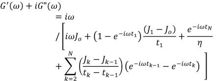
The creep data, however, do only contain information over a limited range of frequencies. The maximum frequency is defined by the resolution (i.e. response time for the first good data point) and the minimum frequency relates to the duration of the experiment. tN-1 < ω <t1-1 represents the frequency window with the valid material information. Data outside of this frequency range are artifact dominated.
This transformation converts temporal strain and stress data sets into oscillatory rheological variables such as G*, phase angle, G’, G”, etc.. The transformation calculates the fundamental frequency from the maximum sampling time and evaluates the harmonics up to the user defined limit (Default is 100). Note that the maximum number of harmonics depends on the sampling rate (Nyquist criterion). For more details on the DFT refer to the TAI product note "APN007_V2 Analyzing Evaluating Oscillation Data." The Arbitrary wave test and any other transient test mode can be used to generate the transient strain, i.e. stress data sets for the transformation.
Example: Exponential pulse test.
In the arbitrary wave test mode form enter the following equation:
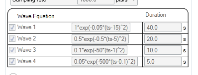
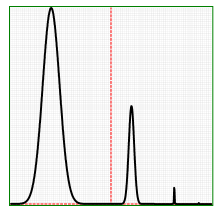
The corresponding strain curve shows three exponential pulses.
The Oscillation (DFT) transformation converts the applied strain and the measured stress using discrete Fourier transformation and displays the results in terms of G’ and G” up to the user defined number of harmonic frequencies. The data will superpose with data obtained from a regular frequency sweep.
Window correlation operates on two transient sinusoidal signals. It is used primarily to follow fast evolving systems and is similar to the ‘fast sampling’ test mode in Oscillation. The difference is that instead of strain and stress, any transient signal recorded during the test can be used. The Window correlation transformation is a post-test operation and correlates the transient signals in a user defined window. When the input strain signal is a continuous sine wave, the window size (number of data points) has to be chosen to match exactly one or an integer number of periods. The window moves along the data set point by point and provides for each data point a complete set of oscillation variables (magnitude and phase for signal 1 and 2, magnitude ratio and phase ratio as well as the real and imaginary part of the magnitude ratio). The new oscillation variables are appended to the same data file starting at the data point that corresponds to the selected window size. Note that this transformation does not generate a new data file.
The transient SineWave test and the Arbitrary test mode are recommended to generate the transient signals. In both cases the strain is the input signal.
This transformation converts and resorts the data using either the WLF or Arrhenius models, and creates a new file at the requested frequency.
This transformation converts and resorts the data using either the WLF or Arrhenius models, and creates a new file at the requested temperature.