Using FT Rheology

Introduction

The expression "FT-Rheology" has been introduced by Manfred Wilhelm and stands for the analysis of the non-linear rheological response to a sinusoidal deformation using discrete Fourier transformation (DFT).

In addition to the DFT, the FT-Rheology option in TRIOS incorporates a complete software package to analyze and present the non-linear oscillation response to a mechanical perturbation. The FT-Rheology package provides the following features:

• Transformation of the temporal strain and stress functions to the power and phase spectrum. The initial data set has to be generated using a transient sine strain test or any oscillation test in transient acquisition mode. The transformed functions are the strain and stress magnitude and phase.
• Extraction of the fundamental and harmonic frequencies. Calculation of the intensity ratio I_n/1 and the phase j_n, the Fourier coefficients (G’_n, G”_n) and the Chebyshev polynomial coefficients (e_n, v_n), for the selected harmonic number n. Typical non-linear measures such as: S, T, Q, G’_L,G’_M, h’_L,h’_M,… are extracted as scalars.
• Recast the fundamental and harmonic data as a function of the oscillation test parameters w, g, t, and T for plotting and further evaluation purposes.  
• Reconstruct temporal strain and stress for one oscillation cycle from the odd Fourier coefficients.

The FT-Rheology option consists of three transformations, and at each transformation a complete new data file is generated. Like any other transformation, the FT-Rheology transformations can be invoked from the File Manager or from the FT-Rheology menu on the ribbon.

• NOTE: In order to access the FT-Rheology functionality, a separate key is required. Without this key, the FT-Rheology option cannot be used. See Setting TRIOS Options for additional information.

Performing FT-Rheology Transformations

Before any of the FT-Rheology transformations can be used, the appropriate data set has to be selected in the File Manager, or the correct plot has to be selected in the document view. In the File Manager, the FT-Rheology transformations are applied to all the data and all data subsets of the selected file. In the document view, the FT-transformation is applied to the selected data in the selected document only.

Generating Data for FT-Rheology Evaluation

Only oscillation data obtained from the "transient – sine strain" experiment or data from any oscillation test (frequency, time, strain sweep) in transient data acquisition mode can be used with the FT-Rheology option. The variables acted upon are the strain (g(t)) and stress (s(t)).

• NOTE:

1. When the data were generated on the ARES-G2, the transducer displacement [transXducerdisplacement] is required to correct s(t) for compliance and inertia effects. Old data sets without this variable are not transformed.

2. The DHR generates data sets suitable for FT-transformation only in the oscillation time and amplitude mode.

3. The DHR attaches a regular time i.e. amplitude sweep to the transient data sets. The ARES-G2 proves only the transient data sets.

When generating the measured data, make sure that more than one oscillation cycle of data points is acquired. More than 1 cycle of data acquisition is required to obtain spectral data points in-between the integer harmonics. These data points provide information on baseline noise and the significance of the harmonic contributions.

Using DFT to Create the Frequency Spectrum

There are two methods to using DFT to create the frequency spectrum: applying DFT using the File Manager and applying DFT at the document level.

The data variables in the frequency spectrum file include:

• The strain and stress magnitude and phase
• The harmonic intensity (ratio of the magnitude of harmonic n and the magnitude of the fundamental)
• The harmonic number and the harmonic phase (phase referred to the sine of the fundamental stress) for the fundamental frequency
• All of the even and odd harmonics up to selected maximum harmonic

Follow the applicable instructions below.

Applying the DFT from the File Manager

To apply the DFT from the File Manager, follow the instructions below:

1. Load the oscillation data file with transient data. Every data file subset represents one dynamic data point and includes the raw strain/stress data over the selected number of oscillation cycles. The file does not need to be opened in the document view if the complete data file is transformed.
2. In the File Manager, right-click the data file and from the drop-down menu select Transformations > FT To Frequency Spectrum. The FT Rheology Transform pop-up window appears with all the subset data files selected. The fundamental test frequency and the Nyquist frequency are displayed. The Nyquist frequency is the highest frequency that can be resolved in the Fourier transformation. The Overall recommended maximum harmonic value is the harmonic number representing the Nyquist frequency.
3. Choose the maximum number of harmonics you would like to evaluate. For most materials, 15 harmonics are sufficient for the analysis. Note that the higher the harmonic number and the number of raw data points, the longer the computation time of the DFT.
4. Click OK to start the transformation. A new data file is created with the extension –ps (power spectrum). The same extension is added to all the data subsets.

Applying the DFT at the Document Level

To apply the DFT at the document level, follow the instructions below:

1. Load the oscillation data file with transient data. Every data file subset represents one dynamic data point and includes the raw strain/stress data over the selected number of oscillation cycles. Display the desired data sets in the document view and set focus to either the temporal strain or stress in the graph.
2. Select the FT-Rheology tab. Select a section of the curve by left-clicking and dragging the mouse pressed along the curve if only a section of the data set is to be transformed. Note that you should always make the selection such that at least one full cycle of data with the strain starting at the zero crossing is included. If less than one cycle of data is selected, the transformation is not performed. An error message appears and the transformation is aborted.
3. Click To Frequency Spectrum on the FT Rheology ribbon. The FT Rheology Transform pop-up window appears with all the subset data files selected. The fundamental test frequency and the Nyquist frequency are displayed. The Nyquist frequency is the highest frequency that can be resolved in the FT-transformation. The Overall recommended maximum harmonic is the harmonic number representing the Nyquist frequency.
4. Choose the maximum number of harmonics you would like to evaluate. For most materials, 15 harmonics are sufficient for the analysis. Note that the higher the harmonic number and the number of raw data points, the longer the computation time of the DFT.
5. Click OK to start the transformation. A new data file is created with the extension –ps (power spectrum). Only the selected data from the actual view is transformed.
6. For transformation purposes, it is useful to suppress various variables during the transformation:

• Suppress harmonic variables in the fundamental: This is helpful in creating a plot showing the fundamental variables and overlaying the intensity of the higher harmonic contributions. In this case, the intensity ratio is suppressed in the fundamental file.
• Suppress modulus variables in the harmonic: In this case, the Fourier coefficients in the harmonic files are suppressed.

Extracting the Harmonics from the Frequency Spectrum

For evaluation of the non-linear material response, only the odd harmonic contributions are important.

The transformation Extract harmonics extracts the even and odd harmonics into a new file with the extension -ps-o. For repetitive transformation operations on similar data files, it is not required to determine the frequency spectrum. The harmonics can be extracted directly from the experimental file. Enter the maximum harmonic number to extract in the FT Rheology Transform pop-up window. The extension of the new file is -o in order to differentiate from the file extracted from the frequency spectrum. The transformation Extract harmonics can be applied to the complete data file using the drop-down menu in the File Manager as well as on a selected data set via the ribbon in the document view. Proceed in the same way as explained in the section Using DFT to Generate the Frequency Spectrum in order to extract the harmonics.

During the extraction of the harmonics, a number of useful variables and scalars are calculated. These data are typically used to describe the non-linear material behavior. The new variables created are the Fourier coefficients (G’_n,G”_n) and the Chebyshev polynomial coefficients (e_n, v_n). Frequently used non-linear parameters including Q-ratio, minimum strain modulus G’_M and large strain modulus G’_L, minimum shear rate viscosity h’M and large shear rate viscosity h’L are calculated and saved as scalar parameters with each data set.

• NOTE: From a rheological point of view, only the odd harmonics are important because the stress response is assumed to be of odd symmetry with the directionality of the shear strain or shear rate. Use the Hide function to prevent even harmonics to be displayed in the graph.
• NOTE: Even harmonics contributions, although small in respect to the odd harmonics, occur and can be related to secondary flow and edge effects at large strains.

Recasting the Data as a Function of the Sweep Parameters

The extracted files contain harmonic information for one dynamic point only. This is not convenient to view the non-linear information as a function of the oscillation test parameter g_o, w, t, T. Therefore, all the extracted harmonic sub-files are recast into a new file with the information of all data points for the fundamental and each of the harmonics.

The recast functionality is a transformation which acts on the full data set of the extracted harmonic file, and as such, it is only available from the transformation on the drop-down menu in the File Manager.

To recast the data:

1. Within the File Manager, right-click a data file with extracted harmonic information and select FT Recast Harmonics from the transformation sub-menu. A new data file is created with the extension -o-o or -p-o-o. The recast file includes a data set for the fundamental and each harmonic. The scalar variables are condensed in the scalar data set.
2. Use the overlay functionality to view fundamental and harmonic variables in one plot.

Reconstructing Sine Strain

To reconstruct the temporal sine wave data from the calculated Fourier coefficients, select a transformed data file with the extension –ps-o.

1. In the File Manager, right-click the data file, and from the drop-down menu select Transformations > FT Reconstruct Sine Strain. Alternatively, click on the FT Rheology ribbon.
2. The Transform to Sine Strain dialog box appears.
3. Enter the Number of points per 1/4 cycle and click OK.
4. TRIOS creates a data file of the original sine strain data. The data file extension reads -ps -o -rec.

The reconstructed data are the strain, strain rate, stress, elastic (real part) stress, viscous (imaginary part) stress for one cycle. In order to switch between different plot presentations, use the predefined plots under Edit > Predefined variables. The available choices are:

• Stress and viscous stress vs. strain rate Lissajous
• Stress vs. strain rate Lissajous
• Stress and elastic stress vs. strain Lissqajous
• Stress vs. strain Lissajous

Discrete Fourier Transformation DFT

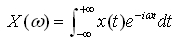
The Fourier transformation converts a periodic temporal signal into a spectral representation in the Fourier domain according to:

If the temporal signal is an array of real numbers of digitized equally distant measurement points, according to x(t)=x(nDt) with Dt=sampling time, n=sample number, N=total samples, Df the frequency resolution in Hz, then:

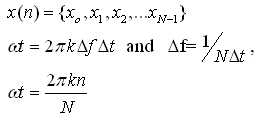
And the continuous Fourier transformation changes to a DFT:

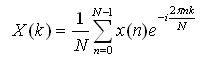
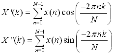
X(k) is a complex number with the real and imaginary part (assuming x(n) is real):

k =1 is the fundamental frequency and all k>1are the harmonics. The maximum harmonic k_max is given by the spectral width. The maximum detectable frequency is f_max= f_ok_max=1/(2Dt) and known as Nyquist frequency.

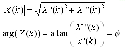
The imaginary and real part of X(k) are used to calculate the magnitude and phase according to:

The DFT in TRIOS provides the magnitude and phase of the stress and strain signals. Since the strain is a sinusoidal input function, the DFT of the strain has a finite fundamental magnitude only; the magnitudes of the harmonics are zero. The magnitude of the fundamental strain is the strain amplitude g. The magnitude of the harmonics of the stress signal is usually represented as a relative magnitude, i.e. harmonic intensity, and is the ratio of the magnitude of the harmonic k and the magnitude of the fundamental: I_k/1=|sk|/|s₁|. The harmonic phase reported is the raw phase of the harmonic referred to the sine of the fundamental stress jk=fk-kf₁.

Fourier, Chebyshev Polynomial Coefficients

In the linear region, the stress response to a sinusoidal strain excitation is also sinusoidal and can be decomposed in an elastic and viscous stress contribution according to:

This equation can be arranged in terms of the storage and loss modulus:

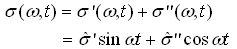
According to Cho et al (2005), the non-linear viscoelastic stress response can also be decomposed in an elastic and viscous stress contribution according to:

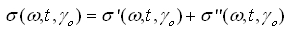
However, the elastic and viscous stress contributions are not linear with respect to the strain or strain rate; a single coefficient G’ (i.e., G”) is not sufficient and a decomposition into higher terms is required. The most direct approach is a decomposition with Fourier coefficients:

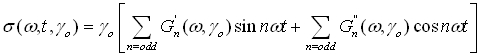
the Fourier coefficients being calculated according to:

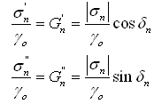
|s_n| is the magnitude of the stress harmonics and d_n the phase referenced to the input strain. Both parameters are direct results from the discrete Fourier transformation.

Another possibility to describe the non-linear viscous and elastic stress is to use Chebyshev polynomials of the first kind. These polynomials are symmetric about x=0, are orthogonal on a finite domain [-1,1] and can easily be related to the Fourier coefficients:

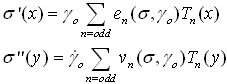
with T_n(x), T_n(y) are the n^th order Chebyshev polynomials of the first kind, and

These functions at each order are orthogonal, and therefore the elastic and viscous Chebyshev coefficients e_n(w,g_o), v_n(w,g_o) are independent of each other. The deviation from the linearity, i.e. n=3 harmonic, can be interpreted as follows. A positive e₃ corresponds to intracycle stiffening of the elastic stress, a negative e₃ indicates strain softening. A positive v₃ represents intracycle shear thickening of the viscous stress, a negative v₃ represents shear thinning. 

In the linear viscoelastic region, e₃/e₁<<1 and v₃/v₁<<1 the equations above reduce to the linear viscoelastic result with e₁→G’ and v₁→G"/w.

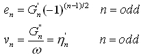
The Chebyshev coefficients in the strain and strain rate domain relate to the Fourier coefficients in the time domain according to:

Non-linear Parameters

The non-linear dynamic mechanical analysis uses a number of non-linear parameters to describe the various aspects of the non-linear rheological behavior. These parameters have been introduced and used by individual researchers, but none of these parameters have been universally accepted. Since these parameters can be determined rather easily from the Fourier coefficients, TRIOS calculates these parameters and stores them as scalars. In the following table, the scalar parameters calculated by TRIOS are listed and commented.

Table of Non-linear Parameters Calculated by TRIOS

Parameter	Definition	Comments	Reference(s)
I3/1	ratio magnitude of 3rd harmonic and fundamental stress	Relative intensity of the 3rd harmonic stress contributions (non-linear monitor)	1, 2
d3	Phase of 3rd harmonic referenced to the input strain	Relates to e3 = –|G3|cosd3 and v3 = (|G3|/w)sind3	1, 4
e3/e1	Ratio of 3rd and 1st Chebyshev elastic coefficient	Relative 3rd order elastic Chebyshev coefficient	4
Q	Q-Ratio =	Coefficient used to characterize branching in polymers	5
G’M	Minimum strain modulus =		4
G’L	Large strain modulus =		4
h'M	Minimum strain rate viscosity =		4
h'L	Large strain rate viscosity =		4
S	Strain stiffening ratio =		4
T	Shear thickening ratio =		4

References

1. Wilhem, M, P.Reinheimer, and M. Ortseifer,“High sensitivity Fourier-transform rheology“, Rheol.Acta 38, 349-356 (1999)
2. Neidhoefer, T., M. Wilhelm, and B. Debbaut, “Fourier transform rheology experiments and finite –element simulations on linear polystyrene solutions,” J.Rheol. 47, 1351-1372 (2003)
3. Cho, K.S., K.H. Ahn, and S.J. Lee, “A geometrical interpretation of large amplitude oscillatory shear response,” J.Rheol. 49, 747-758 (2005)
4. Ewoldt, R.H, A.E.Hosoi, and G.H. McKinely, “New measures for characterizing nonlinear viscoelasticity in large amplitude oscillatory shear,” J.Rheol. 52, 1427-1458 (2008)
5. Hyun, K., E.S.Baik, K.H.Ahn, S.J.Lee, M.Sugimoto, and K.Koyama, “Fourier-transform rheology under medium amplitude oscillatory shear for linear and branched polymer melts’” J.Rheol. 51, 1319-1342 (2007)

© 2014 TA Instruments–Waters LLC | 159 Lukens Drive | New Castle, DE 19720