Performing Time Temperature Superpositioning (TTS) Analysis
There is an equivalence of the effects of time or frequency and temperature on the rheological properties of viscoelastic materials. At low temperatures, a material will behave in a predictable fashion as at high temperature(and the other way around). For example, lowering the temperature of a polymer may proportionately increase the time over which dynamic mechanical responses occur. Rheological parameters in a range of temperatures over modest frequency ranges can be collected and arranged to predict the behavior over a wider frequency range. The TTS option in TRIOS allows sets of frequency-, time-, and temperature-dependent rheological parameters to be shifted horizontally, vertically, or both until they overlap.
A TTS session can be split in several sections: 1) Separating and grouping of experimental data in frequency, time or temperature dependent data sets; 2) Shifting the data sets until they overlap and determination of the shift factors; 3) Creating master curves; 4) Analyzing the shift factors (WLF, Arrhenius).
Selecting data for TTS
Data sets for evaluation using the TTS option can be generated and presented in different formats, for example individual frequency dependent data sets at constant temperature or sets of data depending on frequency and temperature. All data sets selected for evaluation must be loaded into the file manager. There is no need to open the files and display the data.
If the data set is a composite file with frequency and temperature dependent data, the file needs to be separated into individual temperature of frequency dependent data sets.
- Open the desired data file you wish to analyze and load the file into the File Manager. Ensure that the data files have all the same structure (frequency-dependent data set at constant temperature, for example).
If the data file is a composite file:
- Open the File Manager.
- Right-click the data file in the File Manager and select Transformations > Split frequency cycles into frequency sweeps or Split frequency cycles into temperature sweeps to separate the data file into individual files (steps). A document file is added with the data split into frequency or temperature sweeps. The value of the constant variable (temperature or frequency) is appended to the step name.
- The TTS session can be opened in the current document or in a new document. To open a new overlay document, with the Results tab selected in the File Manager,right-click within the File Manager and select New Overlay Document.
- Send the data files you wish to shift to the same graph in the document. You can either select the files and drag and drop them into the empty document, or select the Send To Graph command from the drop-down menu. A graph opens automatically when the first data file is dropped or send to the new document. The tab name changes to Step overlay.
- Select the parameters on the Y axes you wish to shift.
Using the TTS Wizard
Once suitable data has been loaded, and graphed, the TTS ribbon becomes active. The TTS Quick Wizard easily and quickly steps you through the procedure to generate a Master Curve.
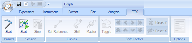
- Click Start
 on the Wizard toolbar.
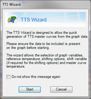
- A TTS Wizard dialog box displays. Click Start to begin the Wizard.
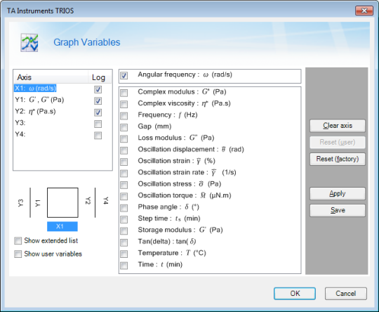
- Select the graph variables and then click OK.
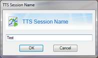
- Choose a TTS session name and then click OK.
- Make your TTS Options selections and then click OK.
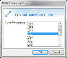
- Select the Reference Curve and then click OK.
- Select the temperature or frequency:
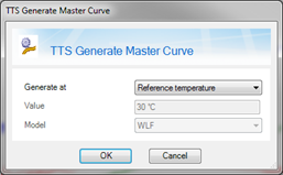
- To use the Reference temperature that was selected in the step above, select Reference temperature from the drop-down list.
- To set a different value, select Explicit temperature from the drop-down list, and then enter the temperature in the Value field. Then select the Model (WLF or Arrhenius) from the Model drop-down menu.
- To set the Explicit frequency or Explicit angular frequency, make the appropriate selection from the drop-down menu, then enter the value (Hz or rad/s, respectively) and select the Model (WLF or Arrhenius) from the Model drop-down menu.
- Click OK. The Master Curve is generated.
Using TTS
- Click TTS tab > Session toolbar > Start. A window for prompting for the TTS session name appears. Enter a session name and click OK. The session name is also the file identifier.
- To ensure that TTS executes properly, select Options and review the settings for the shift algorithm.
- Select one variable (it does not matter which) to mark a data file as reference file. The legend identifies the overlay by the shift variable (temperature or frequency) in the legend table. Upon selection of a text segment in the legend, the corresponding curve in the overlay graph is highlighted. Selecting a curve in the graph shows a box around the corresponding text item in the legend. Select Curves toolbar > Set Reference to mark the selection. The file selected is now the reference and all the data files are shifted to overlay with the reference.
- After selecting the reference curve, you can begin to shift the curves. Verify settings from the Options toolbar before shifting the curves.
- To automatically shift the curves, select Shift from the Curves toolbar. The shifted data appears on the graph. If you want to fine tune the shifted data, use the option below to manually adjust the curve position.
- Two manual shifting procedures are possible.
- Left-click the curve you want to shift. Hold the mouse button down while dragging the curve along the x axes. Note, it is not possible to drag the curves of the reference data file. Note also that all the variables of the selected data file are shifted and rheological consistency remains conserved.
- Left-click the curve you want to shift. Shift the curves fast or slow along the x axes by activating the blue arrows with a mouse click. Click Toggle to activate the vertical shift arrow buttons.
- X and Y shift can be reset individually by clicking Reset Y and Reset X. Automatic and manual shifting can be combined to optimize the shift.
- When the X and Y shifts have been completed, click Masterto generate a new file with the master curve. The master curve file contains only the variables selected in the graph when opening the TTS session. Note that the mastercurve file can be deleted any time during a TTS session by selecting the master curve step and clicking Delete from the drop-down menu in the File Manger.
- End the TTS session by clicking Stop from the Session toolbar. A window appears requesting whether you wish to save the shift factors or not. This window only appears if you selected this option in the Options menu. Note that the TTS shift file step can always be deleted after the TTS session has been closed.
Evaluating Shift Factors
The results generated by the shift algorithm are reported in the shift factor spreadsheet, shown below. In this example, the results are obtained from shifting a series of frequency sweeps.
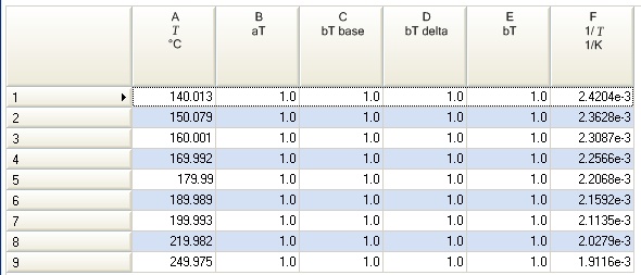
- The sort parameter is the original data set scalar: either the temperature or the frequency, depending on the shifted data sets (frequency or temperature sweeps).
- The aT is the logarithmic value of the horizontal shift factor, i.e. the number by which each x-axis was multiplied in order to shift the data. When the TTS session is started, all horizontal shift factors (aT) are set to one.
- Several bT variables are available:
- The bT base is the logarithm of the vertical shift which is due to temperature/density compensation, i.e. the number by which each y-axis value was multiplied in order to compensate for temperature/density effects. The compensation is always done based on a density of 1.0. Editing the density in the density column will change the bT base variable accordingly. The compensation factor is given as riTi/(rrefTref). The index i refers to the data set being shifted and the index ref to the reference data set. When Y-shift base is set to none in the shift settings, the bT base variable is one.
- The bT delta is the vertical shift generated by the shift-algorithm when horizontal and vertical shifting are allowed, minus the Y-shift base. This variable remains zero when only horizontal shift is allowed.
- The bT is the producy of the bT base and bT delta.
The shift factors can be fitted to a model, either during the TTS session or after the TTS session has been closed (assuming the TTS shift factors were not removed). Proceed as follows:
- Select the shift factor graph.
- Select the Analysis tab.
- Select the curve you which to fit (typically aT vs. T) and set the limits (see details in Analysis help).
- Select the model.
- Refer to Analysis help for details.
Shift Factors Toolbar
The Shift Factors toolbar (shown below) provide access to left-right and up-down shift functions, as well as provides the ability to remove the shifting factors per axis.
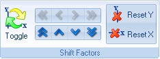
- Toggle switches between vertical and horizontal switching.
- The double shift arrow indicates a change in magnitude of 0.1, while single shift arrow indicates a change in magnitude of 0.01.
- The Reset Y and Reset X functions arrange the respective curves back to their original position.
Options Toolbar
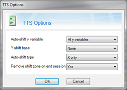
Click Options  to display the TTS Options dialog box (shown below). These settings are used during shift factor operations.
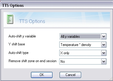
Auto shift y variable
Select from the Auto shift y variable drop-down list when performing an automatic shift. There are two different modes:
- Selected y variable only – Only the variable currently selected on the graph is used to calculate the optimum shift. This may be useful if other variables on the graph are not suitable for inclusion when optimizing the shift.
- All y variables –All variables in the plot are used in the minimization of the residual to optimize the shift
Y shift base
- None – No vertical shift.
- Temperature – The vertical shift base is calculated as Tref /T.
- Temperature*density – The vertical shift base is calculated as Trefrref/Tr.
r is the density, T is the Temperature.
Autoshift type
- X only – Shift algorithm horizontal only. Vertical shift base is calculated as selected in Y shift base. The vertical shift “Y shift base” and “Y shift” are identical.
- X and Y – Shift algorithm horizontal and vertical. “X shift” and “Y shift” are obtained from the minimization routine. The vertical shift base factors are calculated based on the Y shift base option selection. “Y shift” and “Y shift base” can be different. This is usually due to experimental errors in the modulus. Shifting on the tan d variable only removes the experimental errors of the modulus from the shift. In this case the superposition of the moduli or the viscosity is less consistent.
Remove shift zone at the end of the session
- No – The Shift factor data remain after the TTS session closes.
- Prompt – TTS prompts for information whether removing or keeping the shift factors before closing the session.
- Yes – The shift factor data are removed after the TTS session closes.