Bicone Interfacial Accessory

Overview

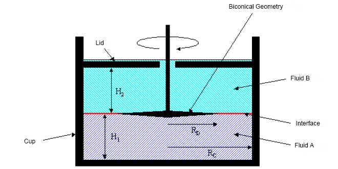
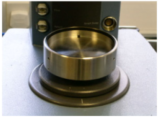
The bicone interfacial accessory is mainly used to determine the viscosity of the interface between two liquid phases. The stator is a circular cup with removable lid, the geometry is a thin, biconical disc (shown below). For chemical inertness, and to reduce the meniscus effect, the cup and lid are constructed from poly(tetrafluoroethene), PTFE, and the geometry from stainless steel.

1. NOTE: Fluid A is the more dense fluid, Fluid B the less dense fluid, R1 is the disc radius, R2 is the cup inner radius, H1 is the lower fluid depth, and H2 is the upper fluid depth. For correct operation, H1 should equal H2.

It is important that the cup and disc are aligned concentrically, and the base with Smart Swap™ connector into which the cup sits has been designed to ensure this. Normally, the cup should be exactly half filled with the more dense sample fluid, and filled to the top with the less dense fluid. The disc is placed at the interface of the two fluids. A mark has been lightly inscribed on the inside of the cup to indicate when it is half full.

Dimensions

• Cup
• Depth: 45 mm
• Inner diameter: 80 mm
• Volume: 226 cm³ (approximately)
• Material: PTFE

• Geometry
• Disc diameter: 68 mm
• Bicone angle: 10°
• Inertia: 32.4 μNm s² (approximately)
• Material: BS970-303 S31 grade stainless steel

• Interfacial surface area: 1395 mm²
• Geometry gap with disc edge level with the cup half full mark (22.5 mm): 19,500 μm (approximately)
• Temperature control: Ambient only

Back to top

Experimental Procedure and Data Treatment

The calculation of the interfacial viscosity for the general case is complicated and can only be solved using numerical procedures [S-G. Oh and J.C. Slattery, Journal of Colloid and Interface Science, 67, 516 - 525, 1978]. However, if the first order assumption is made that the contributions from the three phases are independent of each other, then the calculation becomes relatively straightforward. The contributions from each of the two bulk fluids can be determined separately, and the interfacial contribution can be obtained by subtraction of these from the total contribution.

To do this, the cup is filled completely with one of the fluids, and the geometry is set to gap of 19,500 μm, so that the disc edge is level with the half full mark. The viscosity contribution is determined over the range of shear rates of interest. The process is repeated for the other fluid, and for each shear rate the contributions for the two fluids are added together. The total will be twice that of the upper and lower fluids combined when they each occupy half the cup volume. This value can therefore be halved and subtracted from the total contribution, obtained in the presence of the interface, to give the viscosity due to the interface. A two-dimensional analog of the concentric cylinder geometry is used to calculate the interfacial rheological properties. Details of the analysis are given below. A similar procedure can be used to obtain the dynamic properties of the interface.

Back to top

Operation

Setting up the Interfacial Bicone Accessory

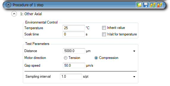
Follow the instructions below to set up the rheometer with the bicone interfacial accessory:

1. Raise the instrument head, and attach the cup holder to the rheometer using the Smart Swap connector, as shown below.

2. Place the cup in the holder, without the lid. Insert the geometry shaft through the hole in the cup lid, and attach the geometry to the rheometer spindle. Lift the lid and fix in the upper position, as shown below, by passing the slots in the lid over the lugs attached to the geometry shaft, and rotating the lid. Use the knurled grips to handle the lid, to avoid touching the under surface; these can either be gripped manually, or using a pair of fine-nosed pliers.

Zeroing the Gap

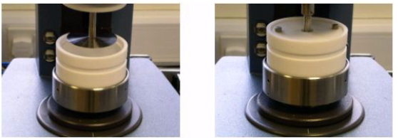
Lower the instrument head until the bicone is within the cup, but is clear of the cup lower surface. Lower the lid to sit in the groove on top of the cup. Zero the geometry gap in the usual way. Note that at the zero position the lugs on the geometry shaft will be approximately 2 mm clear of the lid.

Mapping and Other Calibrations

Rotational and oscillatory mapping and other calibrations, for example of the geometry inertia and bearing friction, are best carried out at this stage. Set a gap of 19500 mm, and perform the mapping and calibrations in the usual way.

Determining Each Fluid's Contribution

Follow the steps below to determine the contribution from each bulk fluid.

1. With the gap set at 19500 mm, fill the cup with sample Fluid A until the fluid is just above the lower edge of the groove on top of the cup. Gently lower the lid. The fluid should overflow from the annular gap between the lid and the geometry.
2. To obtain the sample viscosity, use a Flow procedure and apply the required shear rate (or angular velocity) or range of shear rates. It is usually preferable to use a Steady State Flow procedure for this, but the details will depend on the sample, and the reasons for conducting the experiment. This procedure gives the viscosity contribution of fluid A, η_Acalibration(ẏ), at shear rate .
3. To obtain the sample linear viscoelastic properties, use an oscillation procedure and apply the required strain or range of strains, at the frequency of interest. This will give the storage and loss modulus contributions of Fluid A, G’_Acalibration(ω) and G’’_Acalibration(ω).
4. After running the procedure, raise the instrument head, and remove, clean and replace the cup. Repeat the procedure for the sample Fluid B, to obtain η_Bcalibration(ẏ), G’_Bcalibration(ω) and G’’_Bcalibration(ω), then remove, clean and replace the cup.

Finding the Interface Position

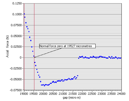
Use the following procedure to fill the cup and find the interface position:

1. Raise the instrument head to the backoff distance then lift and fix the lid.
2. Fill the cup to the half full mark with the more dense of the sample fluids.
3. Set a gap of 24000 μm and lower the lid.
4. Ensure that the Zero axial force before run box is checked under Options > AR > Conditioning.
5. Use an axial test similar to that shown below.

6. Plot the results as normal force against gap. When the geometry is at the interface, the normal force passes through zero. To establish this point, the graph grid and cursors can be used, as shown below.

7. Determine the point at which the axial force passes through zero. This is the position of the interface, which should be at a gap of approximately 19500 μm. Adjust the fluid volume to obtain this gap. Keep in mind that 1 mL of fluid changes the level by about 0.275 mm.
8. When the interfacial position has been identified, manually set the gap to that position (in the example shown on above, to 19527 μm).
9. Lift and fix the lid. You may find it convenient at this stage to add any surfactants to be used.
10. After addition of surfactant, gently add the less dense fluid until the lower edge of the groove on the top of the cup is just covered, then lower the lid gently. The upper fluid should overflow from the annular gap between the lid and the geometry shaft. The viscosity of the total system including the interface can now be measured.
11. Run the Flow or Oscillation procedure to determine the contributions of the two bulk fluids, described above, to obtain the total viscosity contribution η_total(ẏ), or modulus contributions G’_total(ω) and G’’_total(ω) as described.
12. Calculate the interfacial viscosity or dynamic properties as in the next section.

Back to top

Analyzing Results

Calculation of the Interfacial Contribution to the Torque

The interfacial contribution to the torque, η_interfacial(ẏ) at a particular shear rate is calculated by subtracting the contributions of the two bulk fluids, A and B from the total viscosity contribution for the system at that shear rate, i.e.:

η_interfacial(ẏ) = η_total(ẏ) - η_A(ẏ) - η_B(ẏ)

η_A and η_B are obtained from the calibration routine described above. Note that these are not the actual viscosities of the two fluids, they are the contributions that their viscosities make to the total resistance to flow. But η_A (ẏ) is half the viscosity contribution obtained at for fluid A from the calibration routine, and η_B is half that obtained for fluid B, since for the calibration routines the cell is filled with the relevant fluid, whereas for the interfacial measurement it is half filled with Fluid A and half with Fluid B, i.e.

η_A (ẏ) = η_Acalibration(ẏ) / 2 and η_B (ẏ) = η_Bcalibration(ẏ) / 2

Three data points are therefore needed for each shear rate used:

• The calibration data point for Fluid A
• The calibration data point for Fluid B
• The data point for the total system

Then:

η_interfacial(ẏ) = η_total(ẏ) - [η_Acalibration(ẏ) + η_Bcalibration(ẏ)] / 2

If the interfacial shear stress is required, it can now be calculated:

σ_interfacial = η_interfacial x ẏ

Calculation of the Interfacial Linear Viscoelastic Properties

The calculation of G’_interfacial(ω) and G’’_interfacial(ω) can be made in a similar way to the calculation of hinterfacial. The properties of complex variables allow us to consider the in-and out-of-phase components of Fluids A and B and the interface separately. Then:

G’_interfacial(ω) = G’_total(ω) - [G’_ACalibration(ω) + G’_BCalibration(ω)] / 2

G’’_interfacial(ω) = G’’_total(ω) - [G’’_ACalibration(ω) + G’’_BCalibration(ω)] / 2

Other variables can now be calculated if required, for example:

|G*_interfacial(ω)| = {[G’_interfacial(ω))]2 + [G’’_interfacial(ω)]2}0.5

δ = atan [G’’_interfacial(ω)/G’_interfacial(ω)] σ_interfacial = |G*_interfacial(ω)| x γ

Back to top

© 2014 TA Instruments–Waters LLC | 159 Lukens Drive | New Castle, DE 19720